A simple function: y = x²

I’ll start with the thing I encountered first, the Mandelbrot set, and will focus on key takeaways even if you’re not too fascinated by the math, with focus on applied relevance. Wish me the energy to keep up the effort. Consider something you probably already know: the simple formula y = x². Here’s a plot of the function, in case you don’t remember. The function maps each point on the x-axis, which is the real numbers in this case, onto the y axis. As you probably also remember, 0*0 = 0, and 1*1 = 1.

Let’s assume that 0 and 1 have some special meaning for further considerations. 0 may stand for a phenomenon that vanishes, the void. 1 stands for something that is stable, and appears to have an existence. In computer science, 0 and 1 may stand for “on” and “off”, also called Boolean variables. That’s not too important here, we just want to get your thinking started.

The Principle of Recursion

Now let’s do something mean. Instead of mapping all values on the x-axis, let’s assume we start with just one value on the x-axis x₀. We calculate y = x². If we have y, we do the same with this y again. And again, and again. Thus, we get the general formula x_n+1 = x_n². Once we have chosen our initial value x₀ to feed into the equation, we can put the result into the formula again endlessly, also called recursion. Of course, we won’t do it endlessly in practice, or the computer may just hang. We’ll limit the number of steps, but more on that later.

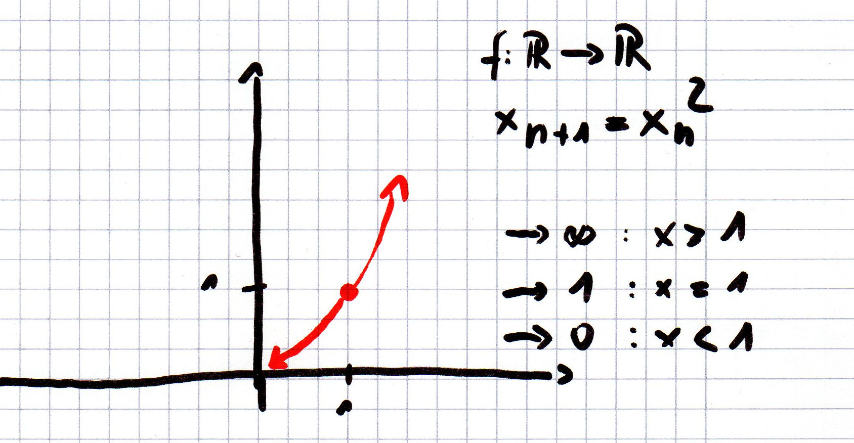
The function can do only three things we send it into recursion. If we picked a starting value that is 1, it stays 1. 1*1 = 1, no matter how often we do that. If we, however, start with 0.5, then we will get 0.25 in the next generation. If we stuff 0.25 in again, we get 0.125, and so on. The number will get smaller and smaller and finally approach 0. If we pick a number that is greater than one, for example 2, the next value will be 4, then 16, and so on. The value will grow towards infinity. Thus, we have three possibilities. Either the value becomes infinitely small and vanishes into zero, it becomes infinitely larger and vanishes into infinity, or it simply stays one. In this case, 1 appears to be a stable state between zero and infinity.

Recursion with Complex Numbers

Now let’s be even meaner. Let’s not do that with rational numbers, but go 2-dimensional. And since we want to have 2-dimensional numbers, not simply vectors, we’re going to pick complex numbers. Interestingly, the function then also can do exactly three things. But since we’re in two dimension, our stable state is no longer a point, but it has become a circle.

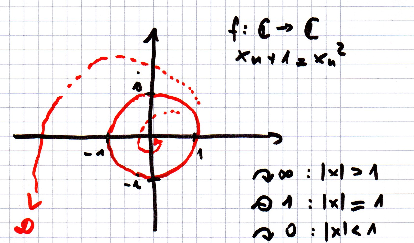
Nevertheless, if s the size of x, also called |x|, is 1, it will stay 1 if we re-enter it into the function. That means, the point we get out of the function and feed back into it will rattle around on the circle with radius 1 from the origin endlessly, until we get tired of computing. Likewise, if the size of the number is smaller than one, it will approach 0. Similarly, it will spiral into 0. That’s due to the weird math of complex numbers. Just believe me. Complex numbers are spinners, when you multiply them. If the size of the number we picked for x₀ is greater than one, it will spin off into infinity. All boring stuff until now, but there are already important takeaways:

:: 1. If something stays the same, it does not mean that it must be static. There may be an underlying dynamic that maps the state into itself endlessly, unless somebody changes the equation.

:: 2. That underlying dynamic does not need to be continuous or linear. It can consist of discrete steps.

:: 3. Attracting and repelling forces can be modelled very easily, attractors and repellers appear to be very basic phenomena in complex systems that occur again and again. Rather than in categorical dichotomies, try to explain a phenomenon with attraction and repulsion. As everything is dynamic in the real world, you will likely have a better fit.

Dynamic Circles

You can stuff any discrete value into the function y = x². If its size is one, it will stay one, although the number you get will be a different one each time … almost.

If you start with 1+0i, then the value will stay 1+0i every time. That’s just the one-dimensional case we had above. But if you start with 0+1i, which also has length 1, you get -1+0i in the next step. And if you square that, you’re back at 1+0i, and you’re done spinning, it stays 1+0i. You may, however, start with sin(1) + cos(1)i. That complex number also has the size 1. Just believe me :) Below is a plot of the first 20 points of the recursion. And yet it moves :) The more steps of the recursion you calculate, the more dense the circle appears.

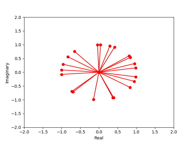
:: 4. Even if you see something like a circle, it may not be as static as you think it is. The underlying dynamics may be hopping from point to point in discrete and rather erratic manner, creating the impression of a continuous circle.

Now let’s make this formula a minimum more complicated. Until now we have only investigated x_n+1 = x_n². Now we’ll try something revolutionary like x_n+1 = x_n² + c. We simply add a small constant. What happens? The first guess may be, that this circle is simply offset, like this:

But as my comment indicates, this is not what happens. The point 1.5 + 0i should stay on the circle, but of course it does not. It flies off towards eternity. In fact, it becomes very difficult now to find points that stay on the boundary and neither drift towards 0 nor become infinity. What does its shape even look like? Is it still a circle? Of course, I have already invalidated that possibility. But what does it look like?

Shapes of a Fractal Boundary

It looks like the left of these pictures if we assume c = 0.2 + 0i as a starting value (you can click on it for a larger version). The boundary is not circular at all anymore. At c = 0.5, it looks like it has vanished in the second graphic. And at c = 0.3 + 0i, i.e. between the two we get the nice graphic on the right. The circle has dissolved into a monster. Or better: a fractal. All three graphics are examples for fractal boundaries. The color represents the number of recursion steps it has taken until a particular value is exceeded, for example, x_n+1 > 4.

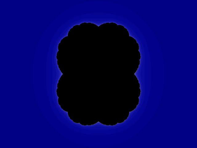
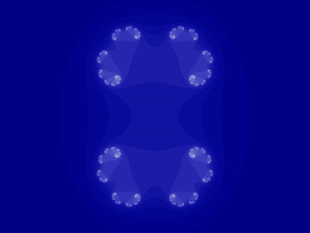
No matter how far we zoom into it, the boundary stays all ragged and torn up, as you can see below on the left. At point c = 0.4 + 0.3i we get the nice snowflake on the right.

These graphics display what is called Julia sets. Apart from being nice pictures, there are more important takeaways:

:: 5. Even if something looks smooth on the surface, it may be indefinitely ragged and torn. If something looks smooth and continuous, it’s more likely an artefact of our perception than a feature of nature. You need better glasses. In nature, everything appears to be ragged, no matter how large we magnify.

:: 6. If your theory relies on smooth and linear math or relationships, you are most likely making hidden assumptions, and your model is only valid within those assumptions. Try to find them, and state them clearly.

:: 7. For complexity to emerge, you don’t need much. The simple formula x_n+1 = x_n² + c can create an enormous amount of complexity. You only need to repeat a simple step over and over, feeding the results into itself.

:: 8. Don’t look for complicated formulae. Look for simple patterns that are used on themselves over and over again. The simpler it is, but the required complexity of properties can still emerge from it by recursion, the more likely you have found something profound.

Benoit Mandelbrot’s Discovery

Mandelbrot wanted to know the influence of c in this equation. He was interested in what the shape looks like that determines whether this Julia set is connected, or dissolves into the cloud and snowflake-like structure that is called Fatou dust (the inverse of the Julia set). Thus, he created an image that combines all possible Julia sets. To do so, he simply mapped the function x_n+1 = x_n² + c on every pixel of the plane, and used the pixel coordinates as c, to see how fast it converges or diverges. The corresponding picture can be seen below. The point 0 +0i is in the centre of the main cardioid body of the shape.

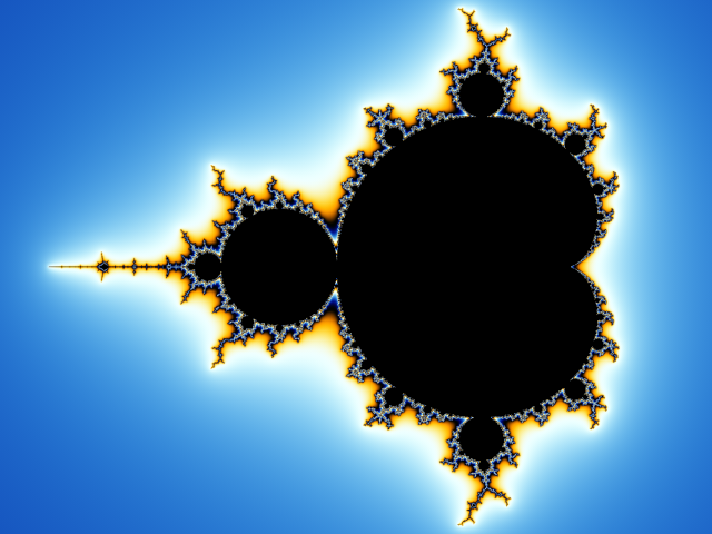
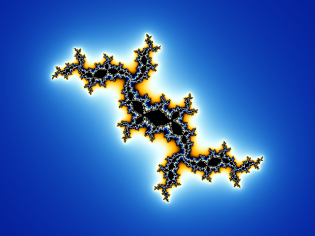
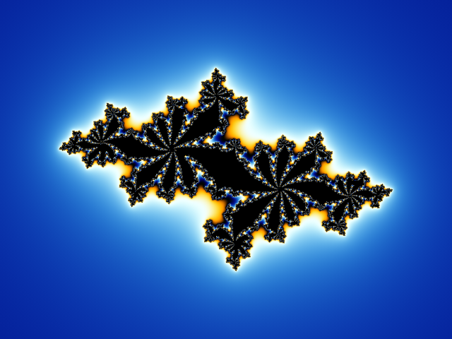
There it is: The Mandelbrot set. My first love and inspiration. Mandelbrot’s initial picture was not as sophisticated as this, but rather an ASCII-printout with asterisks and blanks. It can be found here. However, this shape was clearly visible. As a rule, when you pick a value for c from within the black connected body, the corresponding Julia set will look like a connected pool. If you pick it from the outside area, you will see Fatou dust. Remaining within the black centre but traveling along the attached buds will change the shape of the corresponding Julia set profoundly, as can be seen in the following pictures. The more off the main axes one travels, the more split the basin of attraction of the Julia set becomes.

Fractal Boundary in Detail

We’ve already covered a whole lot of principles of chaotic phenomena, but I want to add two more. Let’s go back to the Mandelbrot set, the first thing I (and many other people) played with. Zooming into the set one can find many phenomena, but some are characteristic.

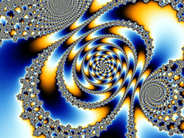
The first recurring theme are spirals. There are a lot of spirals in these images. Spirals represent attraction, where not only series converge, but also the tendency of series to converge itself converges around a point: a meta-structure emerges. This emphasizes the relevance of the basic pattern of attraction and repulsion in looped-discrete phenomena.

In the above image you can see that the interesting stuff, where the complex shapes emerge, are always boundary phenomena. In this case, the complexity arises on the boundary between two attractive basins. The black corpus in the middle of the Mandelbrot set, here seen at the right, is the domain of parameters that do not diverge towards infinity. They resemble the part of values that approach zero in our initial example. The mostly opaque part, at the left, resembles those values who quickly approach infinity. The point that does neither approach zero nor infinity, the point |x| = 1 however, appears to have vanished. It’s broken down into a muddle of complex shapes, and no matter how deep we dig, it’s true location is always one step beyond us.

:: 9. Complex shapes emerge as boundary phenomena between two competing domains of attraction.

Anything interesting (because complex) in nature is a boundary phenomenon. The emergence of complex life, or the emergence of consciousness from the brain’s network are most likely boundary phenomena. The underlying building block that it emerges from can be a lot simpler than the complexity that emerges from it, given enough recursive steps. This boundary is the space, where the recursion no longer approaches zero, but only moderately fast approaches infinity.

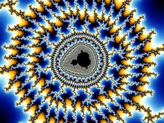
If we dig deep enough, the same basic shape as seen at top level will appear again, and again, in slightly changed forms. The changes are due to influences of the environment. But in principle our senses can see the similarity between the black centre of this image and the top-level shape of the Mandelbrot set in the above image. You can also see this shape in the boundary image above in many places. This principle is called self-similarity.

:: 10. The boundary between the competing two domains is self-similar. If a shape emerges at one point, there is a chance that you will find it at another point. You also may infer of from local observations on the general shape of the system, generalising on its morphology.

This point is important for science. It enables us to infer general laws even from local considerations. There are, however, a couple of caveats: This generalisation does only hold if we don’t tie it to contexts, but only infer general shapes. Science, thus investigates generalities of change, instead of philosophising about the being of instances. Whereas linear approximations form the shapes of probabilistic science and geometry, self-similarity is the principle behind generalisation on looped-discrete phenomena. The same self-similar patterns may emerge at different scales. Thus, conclusions you make may be relevant at different orders of magnitude, but they may not hold in others. While its ok to try to transfer observed patterns to different scales, each scale must be checked for its validity and any extraneous influences that may exert more influence in this context. The pattern may still be visible, but other patterns carry more meaning in this observational cross-section. In this image, the shape of the Mandelbrot set can still be seen and is ultimately behind these complexities. But when judging this picture and its context, the surrounding structures appear to be more relevant for its composition.

Concluding Remarks

I know the above rules still are very abstract, and some of them and their relevance appear to be hard to tackle. Nevertheless, I hope you have at least been infected a bit, and what you read will crawl back up in your mind when you encounter phenomena, either in the outside world or even abstract theories. I hope I could take you at least a part of the way on the journey towards chaos science, to break free from the linear-continuous paradigm of thinking and open a path to find explanations for complex phenomena that transcend linear analysis.

If you liked the pictures only, then here are a few more of my galleries. These formulas are a little more complicated. But they still are one-liners and remain powers, for the most part:

• Expanding the Border
• Digital Exhibition Power & Geometry
• Non-Spirals
• Spirals!
• More of it!
• A lesson in fractal trigonometry

Appendix: Summary of the 10 Properties

1. If something stays the same, it does not mean that it must be static. There may be an underlying dynamic that maps the state into itself endlessly, unless somebody changes the equation.

2. That underlying dynamic does not need to be continuous or linear. It can consist of discrete steps.

3. Attracting and repelling forces can be modelled very easily, attractors and repellers appear to be very basic phenomena in complex systems that occur again and again. Rather than in categorical dichotomies, try to explain a phenomenon with attraction and repulsion. As everything is dynamic in the real world, you will likely have a better fit.

4. Even if you see something like a circle, it may not be as static as you think it is. The underlying dynamics may be hopping from point to point in discrete and rather erratic manner, creating the impression of a continuous circle.

5. Even if something looks smooth on the surface, it may be indefinitely ragged and torn. If something looks smooth and continuous, it’s more likely an artefact of our perception than a feature of nature. You need better glasses. In nature, everything appears to be ragged, no matter how large we magnify.

6. If your theory relies on smooth and linear math or relationships, you are most likely making hidden assumptions, and your model is only valid within those assumptions. Try to find them, and state them clearly.

7. For complexity to emerge, you don’t need much. The simple formula x_n+1 = x_n² + c can create an enormous amount of complexity. You only need to repeat a simple step over and over, feeding the results into itself.

8. Don’t look for complicated formulae. Look for simple patterns that are used on themselves over and over again. The simpler it is, but the required complexity of properties can still emerge from it by recursion, the more likely you have found something profound.

9. Complex shapes emerge as boundary phenomena between two competing domains of attraction.

10. The boundary between the competing two domains is self-similar. If a shape emerges at one point, there is a chance that you will find it at another point. You also may infer of from local observations on the general shape of the system, generalising on its morphology.